Difference-in-Differences in A/B Tests: No Randomizing

When a change does not fit into a user-level coin flip, both obvious readings get the sign wrong. In this guide simulation, comparing the treated group against itself before and after returned minus 0.15 points, comparing treated against control after the change returned minus 0.25 points at a p-value around 3.2 times 10 to the minus 7, and difference-in-differences returned plus 0.25 points, which was the true effect. This guide shows how to build the estimate, what assumption it charges you, and why its standard error is the real minefield: in our placebo run, the conventional reading declared an effect in 29.40 percent of cases where there was no effect at all. It is part of our complete guide to A/B testing and sits next to geo experiments and cluster randomization.

The problem: some changes do not fit a coin flip

A normal A/B test randomizes the user. Half see version A, half see B, and the comparison is honest because the coin flip makes both groups identical in everything, including what nobody measured.

Plenty of changes refuse that coin flip:

• the change is backend, by region. A new carrier that only operates in some states, a local payment method, a tax rule.
• the change is price. Showing different prices to randomized users in the same market is a legal and trust problem long before it is a statistical one.
• the change is brand level. A TV campaign, a sponsorship, a repositioning. There is no version B for half a country.
• the change already shipped. The team pushed it, nobody set up a coin flip, and now somebody wants to know whether it worked.
• the unit is too coarse. With 12 stores or 8 markets, randomizing half leaves statistical power near zero, as we covered in cluster randomization.

In those cases the change arrives through a slice you did not pick at random. And the most natural comparison is then poisoned, because the treated slice already differed from the rest before anything happened.

Worth stating plainly: randomizing is still the preferred option. Blake, Nosko and Tadelis managed to randomize at market level in a paid search experiment at eBay, and the spread between readings was brutal. Ordinary least squares returned a return on investment above 4,100 percent, the same estimate with daily and geographic controls returned above 1,400 percent, and the experimental reading returned minus 63 percent, with a 95 percent confidence interval from minus 124 percent to minus 3 percent. Difference-in-differences is what you use when randomization is unavailable, not a preference over it.

Two wrong readings, and the calculator that confirms both

We simulated a checkout rollout that only worked in some markets. Four numbers carry the whole story:

group	before	after	change
treated markets	3.10%	2.95%	minus 0.15 pp
control markets	3.60%	3.20%	minus 0.40 pp

Two obvious readings fall out of that, and both are wrong.

Reading 1, before and after inside the treated group. From 3.10 to 2.95 percent, minus 0.15 points, minus 4.84 percent in relative terms. Verdict: the change hurt checkout. Wrong, because the whole world got worse over that window.

Reading 2, treated against control in the after period. 2.95 against 3.20 percent, minus 0.25 points, minus 7.81 percent. Verdict: the change hurt checkout. Wrong, because the treated markets already converted lower before.

Reading 2 is the more dangerous of the two, because it passes a significance test. With 260,000 visitors in control markets and 240,000 in treated markets during the after period, paste the four numbers into the calculator:

Control (A)

VisitorsConversions

Variation (B)

VisitorsConversions

Confidence90%95%99%

Control (A) · Rate-

Variation (B) · Rate-

Relative lift-

p-value-

95% CI of the difference-

Two-sided two-proportion z-test. "Not significant" almost always means not enough sample, not that the versions are equal.

Here is what it returns, field by field:

field	control (A)	treated (B)
visitors	260,000	240,000
conversions	8,320	7,080
rate	3.2000%	2.9500%

Result: a difference of minus 0.2500 points, a relative lift of minus 7.81 percent, and a p-value so small the calculator shows only less than 0.0001. Behind that reading sits z equal to minus 5.1117, a p-value around 3.2 times 10 to the minus 7, and a 95 percent confidence interval on the difference from minus 0.3457 to minus 0.1543 points, which the calculator rounds to minus 0.3 to minus 0.2 points. A clean, tight, completely misleading result.

Now run the same calculator on the before period, when there was no change to measure yet: 9,000 of 250,000 in control against 7,130 of 230,000 in treated. It returns a difference of minus 0.5000 points, a relative lift of minus 13.89 percent, and z equal to minus 9.6031, with a p-value so small the calculator shows only less than 0.0001. The “defeat” was already there before any treatment existed. The calculator did not fail: it answered a wrong question with precision.

The estimate, in one line

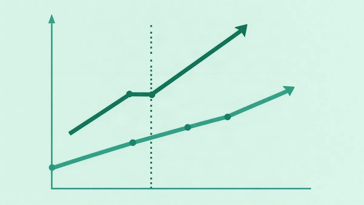
Difference-in-differences does not compare levels, it compares changes:

effect = (treated after minus treated before) minus (control after minus control before)

With our numbers: (2.95 minus 3.10) minus (3.20 minus 3.60) = (minus 0.15) minus (minus 0.40) = plus 0.25 points.

The most useful way to read that is as a four-cell table, because it makes explicit what each subtraction removes:

	before	after	change
treated	3.10%	2.95%	minus 0.15 pp
control	3.60%	3.20%	minus 0.40 pp
difference	minus 0.50 pp	minus 0.25 pp	plus 0.25 pp

The first subtraction, along each row, removes everything fixed about each group: traffic mix, average order value, base quality, dominant channel. If the treated markets always converted half a point lower, that half point leaves the estimate.

The second subtraction, between rows, removes everything that happened to the world in the meantime: seasonality, a holiday, a competitor promotion, a channel algorithm change. In our case, the 0.40 points of decline that hit everybody.

What survives is what happened only to the treated group and only afterwards. That is why the reading works with groups sitting at very different levels: the assumption is not about the level, it is about the change.

The classic example of this reading is Card and Krueger. On April 1, 1992, the New Jersey minimum wage rose from 4.25 to 5.05 dollars per hour. They surveyed 410 fast-food restaurants in New Jersey and eastern Pennsylvania, before and after, and used Pennsylvania, where the minimum wage did not move, as the control group. The relative gain, in their words the “difference in differences” of the employment changes, was 2.76 full-time-equivalent employees, or 13 percent, with a t statistic of 2.03.

The assumption: parallel trends, and how to look at it

The estimate only recovers a causal effect if parallel trends holds: absent the change, treated and control would have moved by the same amount.

That assumption is not testable, because it describes a world that did not happen. But it becomes much more or much less credible depending on what you see before the change. If both series moved together for several periods and only split when the change landed, the assumption is reasonable. If they were already diverging, the reading is dead on arrival.

Three practical checks, all cheap:

1. Plot both raw series. Before any regression. If the chart does not convince you, the number will not either.
2. Run the estimate on placebo periods. Pretend the change landed two weeks before it actually did, using only pre-period data. The answer should be near zero.
3. Run the estimate on placebo metrics. A metric the change could not have touched, say home page bounce rate for a rollout that only altered checkout. If that “improved” too, what you measured was not the change.

The logic is the same as the validation runs we cover in A/A testing: if a method finds effects where none can exist, the method is the problem.

The standard error is the real minefield

The point estimate is arithmetic. The confidence interval around it is where almost everybody gets hurt, and the damage is systematic.

Bertrand, Duflo and Mullainathan surveyed every difference-in-differences article published in six economics journals between 1990 and 2000, 92 in total. Of the 65 that used more than two periods, only five explicitly dealt with serial correlation, and four of those five used a parametric correction that, as they later show, barely moves the needle. On top of that, 80 of the 92 articles had a grouped error problem, because the unit of observation was finer than the unit of variation, and only 36 addressed it.

To size the damage, they generated placebo laws at random in Current Population Survey data on female wages, women aged 25 to 50, from 1979 to 1999, roughly 900,000 observations. Since the laws were fictitious, any significant effect is a false positive, and the correct rate would be 5 percent. Their table:

reading	rejection rate with no effect at all
micro data, ordinary least squares	67.5%
micro data, standard error clustered by state-year cell	44.0%
data aggregated to state-year cells	43.5%
placebo law WITHOUT serial correlation	6.0%
manufactured data with autocorrelation of 0.8	37.3%

The decisive line is the fourth. When they built a law that switches on and off at random, with no serial correlation, the rejection rate dropped to 6 percent. The problem is not the method, it is the combination of a series correlated with itself and a treatment rule also correlated with itself. In their data the first-order autocorrelation of the residuals was 0.51, with second and third order at 0.44 and 0.33, declining far more slowly than a first-order autoregressive process would predict.

We reproduced the same experiment at product scale: 40 markets, 8 treated, 4 weeks before and 4 after, 7,500 visitors per market per week, with autocorrelated noise inside each market.

With a true effect of 0.25 points planted, the estimate came back at 0.2532 points, effectively on the nose. What changes is the standard error:

standard error	value	t	reading
computed per visitor, as if each visit were independent	0.03738 pp	6.775	overconfident
clustered by market	0.05987 pp	4.230	honest
randomization inference, 20,000 draws	empirical cutoff	p-value 0.0006	honest

The standard error clustered by market is 1.6 times the naive one. And the real cost shows up in the placebo run: we repeated the procedure 2,000 times with no effect planted at all, drawing at random which markets would be “treated”.

In our simulation, the standard error computed per visitor declared a significant effect in 29.40 percent of draws with no effect at all, nearly six times the correct rate. Randomization inference returned 5.15 percent, essentially on target.

Randomization inference is the simplest and most robust route, and it is exactly the headline recommendation from Bertrand, Duflo and Mullainathan, because it works regardless of sample size. It fits in three steps:

1. Compute the difference-in-differences estimate with the real set of treated markets.
2. Draw at random, thousands of times, a fictitious treated set of the same size, and compute the estimate for each draw.
3. The p-value is the share of fictitious draws whose absolute estimate matched or beat the real one.

In our case, with 20,000 draws, only 12 matched or beat the observed effect: a p-value of 0.0006.

When permuting is impractical, the two other fixes they tested also work with many units: collapsing everything into two periods, one before and one after, which returned a 6 percent rejection rate; and allowing an arbitrary covariance matrix within each state, which in practice means clustering the standard error by state and also returned 6 percent. Both degrade with few units: in the paper, clustering climbs to 8.5 percent with 10 states and 15 percent with 6, and aggregation climbs to 9.5 percent with 20 states and 31.5 percent with 6.

When the rollout was staggered

So far every treated market entered on the same date. In real life the rollout is usually staggered: one group in week 3, another in week 6, another in week 9. The temptation is to throw everything into a regression with market and week fixed effects and read the treatment dummy coefficient.

Goodman-Bacon showed what that coefficient actually is: a weighted average of every possible 2x2 comparison between timing groups. Some of those are the comparisons you expected, treated against never treated. Others use an earlier treated group as the control for a later treated group, over the window in which the first one is already treated.

In Goodman-Bacon’s terms, when treatment effects do not change over time, the reading returns a variance-weighted average of cross-group effects and all weights are positive. Negative weights only arise when treatment effects vary over time: when already-treated units act as controls, changes in their treatment effects over time get subtracted from the estimate. He notes this does not imply a failure of the design, but it does caution against summarizing time-varying effects with a single coefficient.

The weights, he shows, are proportional to group sizes and to the variance of the treatment dummy in each pair, and that variance is highest for units treated in the middle of the panel. Which means: whoever entered mid-rollout dominates the result, without anyone having decided that.

In practice, for a staggered rollout:

• Do not read a single coefficient. Estimate an effect per period since entry, the event study, and look at the shape of the curve.
• Prefer estimators that use only clean controls, meaning they compare each treated group only against units not yet treated.
• If you must report one number, say who dominated it. A coefficient whose weight sits almost entirely on the middle cohort is not “the effect of the rollout”.

A seven-step difference-in-differences routine

1. Write the question before looking at the data. Which change, which metric, which treated slice, which cutoff date. That goes in the pre-registered analysis plan exactly as it would for a randomized test.
2. Pick the control group by trend, not by level. The best control is not the closest on conversion, it is the one that moved together with the treated group in prior periods.
3. Plot the raw series for both groups before computing anything. If the chart does not convince, the number will not.
4. Run placebo periods and placebo metrics. A large result where no effect can exist kills the reading.
5. Compute the four means and do the double subtraction. That part is arithmetic and takes minutes.
6. Do not use the per-visitor standard error. Use permutation, or cluster by treatment unit, or collapse to two periods. Say in the report which of the three you used.
7. If the rollout was staggered, publish the curve by period, not a single coefficient.

Common mistakes

• Comparing treated and control only in the after period. That is reading 2 in this guide. It flips the sign when levels already differed, and it flips it with a pretty p-value attached.
• Comparing the treated group against itself before and after. That charges the change with everything that happened in the world meanwhile, seasonality and competitors included.
• Picking the control after seeing the result. With ten candidate controls, one of them returns the number you wanted. Picking by pre-trend, and picking first, is what separates measurement from justification.
• Using the standard error your A/B tool offers. It assumes user-level randomization and independence between visits. Here neither holds.
• Assuming a sample ratio mismatch check covers this. SRM compares the sizes of randomized groups. Here nothing was randomized.
• Ignoring composition that shifts mid-window. If the traffic mix of the treated markets changed between before and after for an unrelated reason, the double subtraction does not remove that.
• Treating the result as if it came from a randomized test. Difference-in-differences is the second best option. When you can randomize, randomize, and use the sample size calculator to find out how long that takes.
• Applying the reading when the treatment itself moved the control group. If treated markets stole demand from control markets, you measured the difference plus the spillover, a case of interference between variants.

Make this automatic with Donnu

The most common reason a difference-in-differences reading goes wrong is not the formula, it is the data. The estimate needs the metric by treatment unit and by period, stored under the same definition before and after. A dashboard that only keeps a site-wide total, or that changed the conversion definition midway, does not support the reading, and no statistical sophistication repairs that after the fact.

Donnu stores the outcome by unit and by day with the definition stamped, which turns a difference-in-differences reading into a query rather than a reconstruction. And more to the point, it exists for the case where you can randomize: whenever the change fits a user-level coin flip, that is the route, because it drops the parallel trends assumption and the standard error minefield with it. To find out whether your traffic supports the randomized test before falling back to a quasi-experiment, the sample size calculator answers in seconds, and the significance calculator closes the reading at the end.

References

• Bertrand, M., Duflo, E. and Mullainathan, S. How Much Should We Trust Differences-in-Differences Estimates? NBER Working Paper 8841, 2002, published in the Quarterly Journal of Economics. Source for the survey of 92 difference-in-differences articles published across six journals between 1990 and 2000, of which 65 used more than two periods and only five explicitly dealt with serial correlation, and of which 80 had a grouped error problem with only 36 addressing it; for the Table 2 rejection rates using placebo laws in Current Population Survey data from 1979 to 1999 (67.5 percent for micro data with ordinary least squares, 44.0 percent with clustering by state-year cell, 43.5 percent with aggregated data, 6.0 percent for a law with no serial correlation, and 37.3 percent in manufactured data with autocorrelation of 0.8); for the residual autocorrelations of 0.51, 0.44 and 0.33; and for the rates of the three fixes, including 6 percent for collapsing to two periods and for the arbitrary covariance matrix, degrading to 8.5 and 15 percent with 10 and 6 states under clustering and to 9.5 and 31.5 percent with 20 and 6 states under aggregation. nber.org.
• Card, D. and Krueger, A. B. Minimum Wages and Employment: A Case Study of the Fast-Food Industry in New Jersey and Pennsylvania. American Economic Review 84(4), 1994. Source for the classic example: on April 1, 1992 the New Jersey minimum wage rose from 4.25 to 5.05 dollars per hour, 410 fast-food restaurants in New Jersey and eastern Pennsylvania were surveyed before and after, and the relative gain, the difference in differences of the employment changes, was 2.76 full-time-equivalent employees, or 13 percent, with a t statistic of 2.03. davidcard.berkeley.edu.
• Goodman-Bacon, A. Difference-in-Differences with Variation in Treatment Timing. NBER Working Paper 25018, July 2019 version, published in the Journal of Econometrics. Source for the result that the two-way fixed effects estimator equals a weighted average of every possible 2x2 comparison between timing groups, including those that use already-treated units as controls; for the weights being proportional to group sizes and to the variance of the treatment dummy in each pair, highest for units treated in the middle of the panel; and for negative weights arising only when treatment effects vary over time, in which case changes in the already-treated group effect are subtracted from the estimate, which does not imply a failure of the design but cautions against a single coefficient. vanderbilt.edu.
• Blake, T., Nosko, C. and Tadelis, S. Consumer Heterogeneity and Paid Search Effectiveness: A Large Scale Field Experiment. NBER Working Paper 20171, 2014, published in Econometrica. Source for the contrast between readings: return on investment above 4,100 percent under ordinary least squares, above 1,400 percent with time and geography controls, and minus 63 percent from the experimental variation, with a 95 percent confidence interval from minus 124 to minus 3 percent; and for the geographic design with 68 market areas where ads were suspended, 65 control areas matched on historical serial correlation in sales, and 77 remaining control areas. nber.org.

Read next: Geo experiments · Cluster randomization · Switchback experiments · Randomization unit · Pre-registered analysis plan · Sample size calculator · Leia em português